TLDR: if you skim through and search for a bold text like this paragraph, it might be enough to explain what's going on.
This will be a third post in my series on how to read geonode trees [links at the bottom]. In both previous I recommend reading the node tree ⬅ from right to left, however there is a limitation within which you can read fragments from left ➡ to right: a circular socket 🟣 generates a single value (it's calculated for each tree user once per frame), so it calculates a value based only on inputs from left, regardless of what is connected to the outputs on the right. The only caveat is such a node won't run at all if it's not connected (directly or indirectly) to the Group Output - but it hardly matters, due to the purely functional programming nature of geonodes; there are no side effects (other than performance related: memory usage, execution time, crash risk), so you can reason about your node tree by assuming every such node actually runs.
Since your node tree consists mostly of nodes outputting such 'constants' in the form of 🟢Geometry, it's a good opportunity to try to read it from the left ➡ to right.
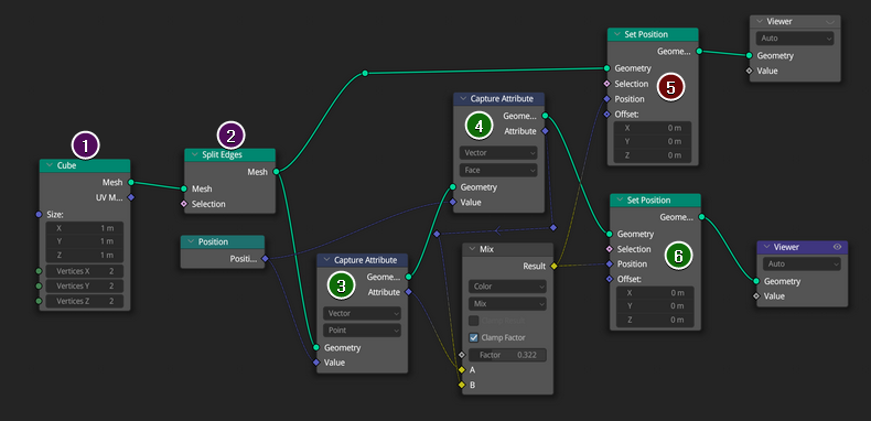
I numbered some nodes to represent steps.
1 Cube
"Cube" node generates and outputs mesh data in the form:
| Index |
Vertices |
Edges |
Faces |
|
coords xyz |
vertex indices |
vertex indices |
| 0 |
-0.5, -0.5, -0.5 |
0, 1 |
0, 2, 3, 1 |
| 1 |
0.5, -0.5, -0.5 |
0, 2 |
0, 1, 5, 4 |
| 2 |
-0.5, 0.5, -0.5 |
2, 3 |
4, 5, 7, 6 |
| 3 |
0.5, 0.5, -0.5 |
0, 4 |
2, 6, 7, 3 |
| 4 |
-0.5, -0.5, 0.5 |
1, 5 |
0, 4, 6, 2 |
| 5 |
0.5, -0.5, 0.5 |
4, 6 |
1, 3, 7, 5 |
| 6 |
-0.5, 0.5, 0.5 |
5, 7 |
|
| 7 |
0.5, 0.5, 0.5 |
2, 6 |
|
| 8 |
|
6, 7 |
|
| 9 |
|
1, 3 |
|
| 10 |
|
4, 5 |
|
| 11 |
|
3, 7 |
|
There's more data than that: UV map (that's face corner domain not even mentioned in the table above), edges contain information like sharpness, faces contain information like material slot index etc. This data also is stored a little bit differently, for example in case of vertex coordinates it's just a one-dimensional array:
>>> import numpy as np
>>> d = C.object.data
>>> coords = [0.0]*len(d.vertices)*3
>>> d.vertices.foreach_get('co', coords)
>>> coords
[-0.5, -0.5, -0.5, 0.5, -0.5, -0.5, -0.5, 0.5, -0.5, 0.5, 0.5, -0.5, -0.5, -0.5, 0.5, 0.5, -0.5, 0.5, -0.5, 0.5, 0.5, 0.5, 0.5, 0.5]
Still, the table is useful to get the point across: It is this table, not some kind of a pointer, handle or name of the geometry, that is passed around in the 🟢 green geometry links. The entire geometry is copied in each link, that's why the following doubles geometry:
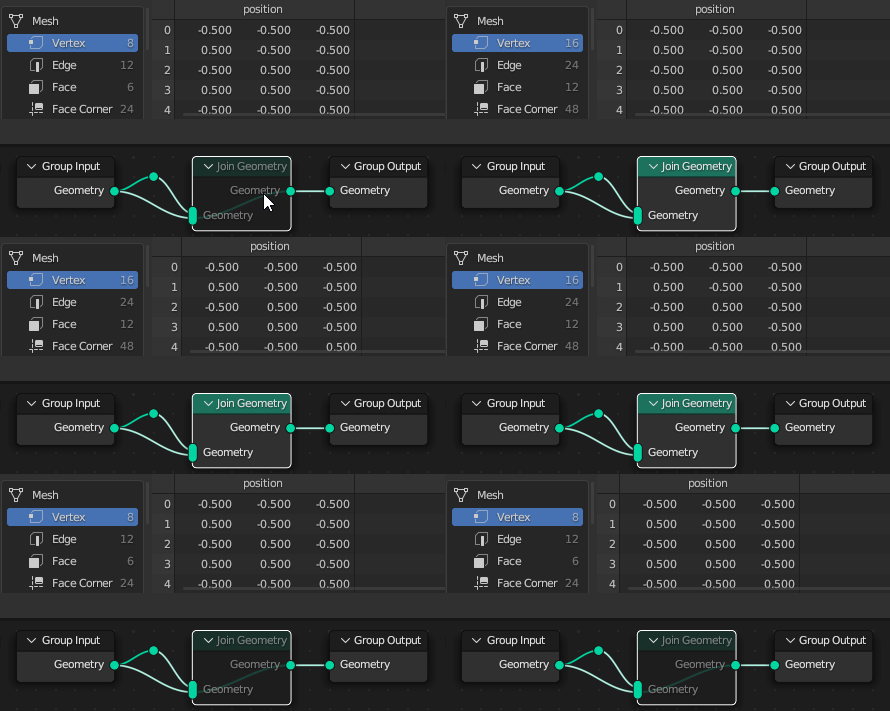
2 Split Edges
"Split Edges" node gets the table, splits all edges and outputs altered mesh:
| Index |
Vertices |
Edges |
Faces |
|
coords xyz |
vertex indices |
vertex indices |
| 0 |
-0.5, -0.5, -0.5 |
8, 10 |
8, 12, 14, 10 |
| 1 |
0.5, -0.5, -0.5 |
8, 12 |
9, 11, 18, 16 |
| 2 |
-0.5, 0.5, -0.5 |
12, 14 |
17, 19, 22, 20 |
| 3 |
0.5, 0.5, -0.5 |
9, 16 |
13, 21, 23, 15 |
| 4 |
-0.5, -0.5, 0.5 |
11, 18 |
0, 4, 6, 2 |
| 5 |
0.5, -0.5, 0.5 |
17, 20 |
1, 3, 7, 5 |
| 6 |
-0.5, 0.5, 0.5 |
19, 22 |
|
| 7 |
0.5, 0.5, 0.5 |
13, 21 |
|
| 8 |
-0.5, -0.5, -0.5 |
20, 22 |
|
| 9 |
-0.5, -0.5, -0.5 |
10, 14 |
|
| 10 |
0.5, -0.5, -0.5 |
16, 18 |
|
| 11 |
0.5, -0.5, -0.5 |
15, 23 |
|
| 12 |
-0.5, 0.5, -0.5 |
9, 11 |
|
| 13 |
-0.5, 0.5, -0.5 |
0, 2 |
|
| 14 |
0.5, 0.5, -0.5 |
13, 15 |
|
| 15 |
0.5, 0.5, -0.5 |
0, 4 |
|
| 16 |
-0.5, -0.5, 0.5 |
1, 5 |
|
| 17 |
-0.5, -0.5, 0.5 |
4, 6 |
|
| 18 |
0.5, -0.5, 0.5 |
5, 7 |
|
| 19 |
0.5, -0.5, 0.5 |
2, 6 |
|
| 20 |
-0.5, 0.5, 0.5 |
21, 23 |
|
| 21 |
-0.5, 0.5, 0.5 |
1, 3 |
|
| 22 |
0.5, 0.5, 0.5 |
17, 19 |
|
| 23 |
0.5, 0.5, 0.5 |
3, 7 |
|
You can imagine this table being put inside the socket:

And once this socket is filled with this table, it is sealed, and the table can't be replaced with another, nor can the contents of this table be changed.
3 Capture Attribute
"Capture Attribute" node is set to operate on points, so it creates a new column of data, and on reach row stores a calculated value. So it sets the context to vert#0 and requests data from the field link, which is connected to Position node, sending -0.5, -0.5, -0.5, then it stores this data on the first row of the new columns, sets the context to vert#1, requests data, Position node reads current vertex position and sends 0.5, -0.5, -0.5 and so on until the column is filled:
| Index |
Vertices |
Vertices |
Edges |
Faces |
|
coords xyz |
anonymous attribute |
vertex indices |
vertex indices |
|
|
ID # 9192631770 |
|
|
| 0 |
-0.5, -0.5, -0.5 |
-0.5, -0.5, -0.5 |
8, 10 |
8, 12, 14, 10 |
| 1 |
0.5, -0.5, -0.5 |
0.5, -0.5, -0.5 |
8, 12 |
9, 11, 18, 16 |
| 2 |
-0.5, 0.5, -0.5 |
-0.5, 0.5, -0.5 |
12, 14 |
17, 19, 22, 20 |
| 3 |
0.5, 0.5, -0.5 |
0.5, 0.5, -0.5 |
9, 16 |
13, 21, 23, 15 |
| 4 |
-0.5, -0.5, 0.5 |
-0.5, -0.5, 0.5 |
11, 18 |
0, 4, 6, 2 |
| 5 |
0.5, -0.5, 0.5 |
0.5, -0.5, 0.5 |
17, 20 |
1, 3, 7, 5 |
| 6 |
-0.5, 0.5, 0.5 |
-0.5, 0.5, 0.5 |
19, 22 |
|
| 7 |
0.5, 0.5, 0.5 |
0.5, 0.5, 0.5 |
13, 21 |
|
| 8 |
-0.5, -0.5, -0.5 |
-0.5, -0.5, -0.5 |
20, 22 |
|
| 9 |
-0.5, -0.5, -0.5 |
-0.5, -0.5, -0.5 |
10, 14 |
|
| 10 |
0.5, -0.5, -0.5 |
0.5, -0.5, -0.5 |
16, 18 |
|
| 11 |
0.5, -0.5, -0.5 |
0.5, -0.5, -0.5 |
15, 23 |
|
| 12 |
-0.5, 0.5, -0.5 |
-0.5, 0.5, -0.5 |
9, 11 |
|
| 13 |
-0.5, 0.5, -0.5 |
-0.5, 0.5, -0.5 |
0, 2 |
|
| 14 |
0.5, 0.5, -0.5 |
0.5, 0.5, -0.5 |
13, 15 |
|
| 15 |
0.5, 0.5, -0.5 |
0.5, 0.5, -0.5 |
0, 4 |
|
| 16 |
-0.5, -0.5, 0.5 |
-0.5, -0.5, 0.5 |
1, 5 |
|
| 17 |
-0.5, -0.5, 0.5 |
-0.5, -0.5, 0.5 |
4, 6 |
|
| 18 |
0.5, -0.5, 0.5 |
0.5, -0.5, 0.5 |
5, 7 |
|
| 19 |
0.5, -0.5, 0.5 |
0.5, -0.5, 0.5 |
2, 6 |
|
| 20 |
-0.5, 0.5, 0.5 |
-0.5, 0.5, 0.5 |
21, 23 |
|
| 21 |
-0.5, 0.5, 0.5 |
-0.5, 0.5, 0.5 |
1, 3 |
|
| 22 |
0.5, 0.5, 0.5 |
0.5, 0.5, 0.5 |
17, 19 |
|
| 23 |
0.5, 0.5, 0.5 |
0.5, 0.5, 0.5 |
3, 7 |
|
4 Another Capture Attribute
Right "Capture Attribute" node works very similarly: it gets the table from above (the one with one anonymous attribute column), and adds yet another column, this time for the face domain. First it sets the context to face#0, asks the field for data, "Position" node hears this request over the field link and given the context is face#0, it sends the position of the face, however it is implemented to obtain it: 0, 0, -0.5. Then the "Capture Attribute" node saves this data, changes context to face#1 and repeats until all faces have been evaluated.
| Index |
Vertices |
Vertices |
Edges |
Faces |
Faces |
|
coords xyz |
anonymous attribute |
vertex indices |
vertex indices |
anonymous attribute |
|
|
ID # 9192631770 |
|
|
ID # 299792456 |
| 0 |
-0.5, -0.5, -0.5 |
-0.5, -0.5, -0.5 |
8, 10 |
8, 12, 14, 10 |
0.0, 0.0, -0.5 |
| 1 |
0.5, -0.5, -0.5 |
0.5, -0.5, -0.5 |
8, 12 |
9, 11, 18, 16 |
0.0, -0.5, 0.0 |
| 2 |
-0.5, 0.5, -0.5 |
-0.5, 0.5, -0.5 |
12, 14 |
17, 19, 22, 20 |
0.0, 0.0, 0.5 |
| 3 |
0.5, 0.5, -0.5 |
0.5, 0.5, -0.5 |
9, 16 |
13, 21, 23, 15 |
0.0, 0.5, 0.0 |
| 4 |
-0.5, -0.5, 0.5 |
-0.5, -0.5, 0.5 |
11, 18 |
0, 4, 6, 2 |
-0.5, 0.0, 0.0 |
| 5 |
0.5, -0.5, 0.5 |
0.5, -0.5, 0.5 |
17, 20 |
1, 3, 7, 5 |
0.5, 0.0, 0.0 |
| … |
Skipping |
the rest |
with dedication |
to |
mouse wheels |
5 Set Position
"Set Position" node iterates over points (here: vertices). For each point it evaluates "Selection" - if it evaluates to *True", the two vector sockets are evaluated and added together, the position of the currently evaluated point is set to the result and the context is moved to the next point, until all points have been evaluated.
⚠ This is the moment when you have to again read the nodes ⬅ from right to left❗
- Set the context to vert#0.
- "Selection" by default is True.
- Evaluate "Position" field.
- "Position" field leads to "Mix" node, so execution goes there. ⬅
- "Mix" node evaluates the "Fac" to be the default
0.322.
- "Mix" then evaluates "A" connected to "Capture Attribute" (3) node, so execution goes there ⬅
- This is the crucial part. "Capture Attribute" node is not a sampling node, it doesn't change context when asked for a value of the attribute. It simply shares the ID of the anonymous [it's like on the Internet, you're never truly anonymous] attribute:
91926317701.
- The execution returns to "Mix" ➡
- "Mix" accesses the anonymous attribute column #91926317701 for the first row (because currently vertex 0 is evaluated). But there is no such column! The mesh data being evaluated is the mesh data passed to the upper "Set Position" (5), which never had this column created. Here are some examples how Blender devs could implement resolving such a conflict:
- crashing Blender,
- displaying a warning ⚠ sign on the top of the "Set Position" (5) node with a tooltip "Can't evaluate nonexistent attribute",
- have AI rewire the nodes internally in hopes it achieves the result the user intended,
- set the value to
NaN or 3 or 4 NaNs for vectors or RGBA colors and maybe -1 for integers,
- set all values to 0;
and they decided to use the last option.
- "Mix" treats "B" similarly to "A" in points 6-9 which this time tries to read from also non-existent column ID#299792458, and also evaluates to <0, 0, 0>.
- "Mix" makes a calculation $(1-\mathtt{Fac})×A + \mathtt{Fac}×B = (1-0.322)×0 + 0.322×0 = 0 + 0 = 0$ giving the same result for each of 3 vector components.
- The result
<0.0, 0.0, 0.0> is sent back through the field ➡
- "Set Position" receives the vector
<0.0, 0.0, 0.0>, adds default <0.0, 0.0, 0.0> offset vector, which results again with <0.0, 0.0, 0.0> - that's where the currently evaluated vert#0 is positioned. Everything is repeated from point 1. except now for vert#1, then for vert#2, vert#3 and so on until #vert23 is evaluated.
| Index |
Vertices |
Edges |
Faces |
|
coords xyz |
vertex indices |
vertex indices |
| 0 |
0.0, 0.0, 0.0 |
0, 1 |
0, 2, 3, 1 |
| 1 |
0.0, 0.0, 0.0 |
0, 2 |
0, 1, 5, 4 |
| 2 |
0.0, 0.0, 0.0 |
2, 3 |
4, 5, 7, 6 |
| 3 |
0.0, 0.0, 0.0 |
0, 4 |
2, 6, 7, 3 |
| … |
… |
… |
… |
6 Another Set Position
This answer's length got out of hand so let's just mention how this time the context goes through a table that actually has two anonymous columns ID#9192631770 and ID#299792458, and in the latter case has to interpolate from faces to vertices, which is simply an average of all faces connected to (built upon) currently evaluated vertex. since non-zero values reside in this column, the "Mix" produces various non-zero colors and the lower "Set Position" (6) node therefore positions the vertices differently
More reading:

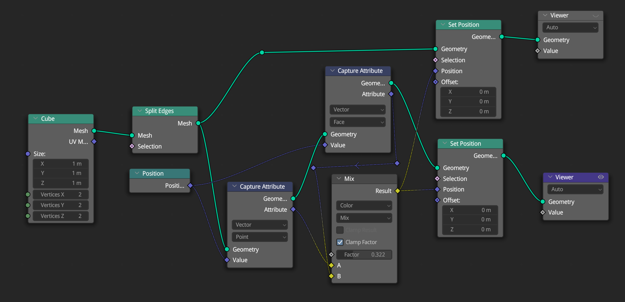


Capture Attributescaptures attributes in the domain you specify in the currently evaluated geometry. Since you are not capturing attributes in the upper geometry (trace the green line backwards from the Viewer node), they cannot be read. If you want to transfer attributes from one geometry to another, you would have to do it withSample Index. $\endgroup$