How to calculate an attribute for each point which depends on every other point

Question

I have come across this difficulty several times while making a node tree and haven't found a solution yet. In general, I want to make a calculation, for example to store as an attribute, for each point in a point cloud. The problem is this calculation depends on all other points in the cloud, not just on itself or on the nearest.

As a concrete example, consider I have some point cloud, with some distribution. For each point P, I want to calculate how many points are within 1m distance of the position 2m below P, and store the result as an attribute. How can this be achieved?

The only time I think I might have come close was when I thought to use Attribute Statistic to sum up the results from a "Less Than" compare node making pair-wise comparisons between the point in question and every other point, but I couldn't manage to make these pair-wise comparisons. I always seem to get a constant result. This is what I would have expected from an Attribute Statistic node, but I don't know how else to achieve this goal. An example node tree is in the screenshot below. In this example, the attribute computes as 0 for all points, though if I use a different seed, it becomes 1 for all values. A higher proportion of seeds yield 1 or higher if I increase the input H Spacing, which has the effect of widening the search radius.

Beyond this specific example, this sort of calculation, if possible, could also be useful for simulations, for example to calculate the net force (such as electromagnetic force) exerted on each point (charge) by every other point. Though the calculation is different, the difficulty is the same.

The electromagnetic force you are mentioning is reminding me this post about gravity: Compute on all points in geometry nodes. — StefLAncien, Commented Apr 29 at 7:33

Gordon Brinkmann · Accepted Answer · 2024-05-02 12:00:47Z

So this is a bit elaborate, but here we go: I use a Repeat Zone with a "Counter" value to go through all the existing points and on each point I use the Sample Index node to calculate the distance from the point with the index "Counter" to all other points.

Then I use the Sum of an Attribute Statistic node to count all points with a distance below a given value and store this sum with a Store Named Atrribute node and use the Selection there to store a value only on that point where the Index is equal to the current "Counter" value.

This way I store on each point the sum of all neighbouring points within a given distance. Or actually all neighbouring points + 1, because the point itself is of course also within this distance. If you don't want that, you could subtract 1 from the value.

Although if (like in your case) you don't want the actual position but a pisition 2 m below - which you can achieve by not taking the position given by the Sample Index node, but the position minus (0, 0, 2) of course - then this subtraction of the original point might not be necessary...? Anyway, I just tried to show a basic way how to store data on points depending on all other points. There are then many ways to manipulate the data in one way or another.

In the beginning of my nodetree I use Distribute Points on Faces to distribute points on a grid, however those have to be converted to vertices or otherwise the Store Named Attribute will not store the values within the Repeat Zone (but you can store on points outside of a Repeat Zone, so I'm not sure at the moment if this is a bug or if the zone simply requires a mesh i.e. vertices instead of a point cloud). If you need them as points, you can put a Mesh to Points node after the Repeat Zone, the points will keep the data stored on the vertices before.

_{(Note: The problem having to use vertices instead of points and therefore the points to vertices conversion was an inadvertence on my behalf, I did not change the Domain Size node to Point Cloud.)}

Nodetree:

An alternative to the Attribute Statistic node would be to simply count up the values within the Repeat Zone. This has the advantage that less computing power is required as the sum does not have to be recalculated for all points with each run:

_{(Tested with Blender 4.1.1: in this case, Points to Vertices is not required)}

What I have done additionally just for visualization purposes is instancing a circle with the radius of the threshold distance on a single vertex chosen by the index, this way you can compare if the number of vertices withing this radius matches the sum stored at this index. For this example setup I have everything on a flat plane so that it is optically better comprehensible, but of course the distance calculation works in 3D space as well.

Example where I instance the circle on the vertex with index 1: the "sum" attribute shows 3, so there should be (and there are) three vertices within the circle around vertex #1:

Blend file:

This works, though it can be slow with more points. Also, I believe it only worked with meshed in your case because the "Domain Size" node used to calculate how many iterations to perform is set to "Mesh", not "Point Cloud". — Érico Patto, Commented Apr 28 at 19:47
@ÉricoPatto Oh damn, you're right I did not switch the Domain Size... My bad, most of the time I never use it so I did not pay attention to it. I agree it might be slow with lots of points but I did not find a more effcient way. Perhaps someone else might know a better way. — Gordon Brinkmann, Commented Apr 28 at 21:32
If I could make a suggestion for improvement here: If you replace the node Attribute Statistic with the following setup, performance can be greatly improved: i.sstatic.net/FypgskvV.png — quellenform, Commented May 2 at 10:36

StefLAncien · Accepted Answer · 2024-05-05 12:35:18Z

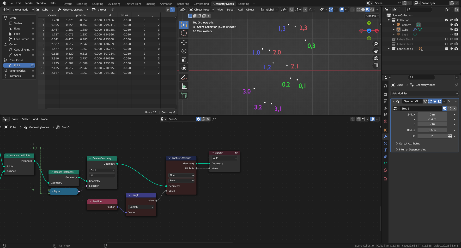
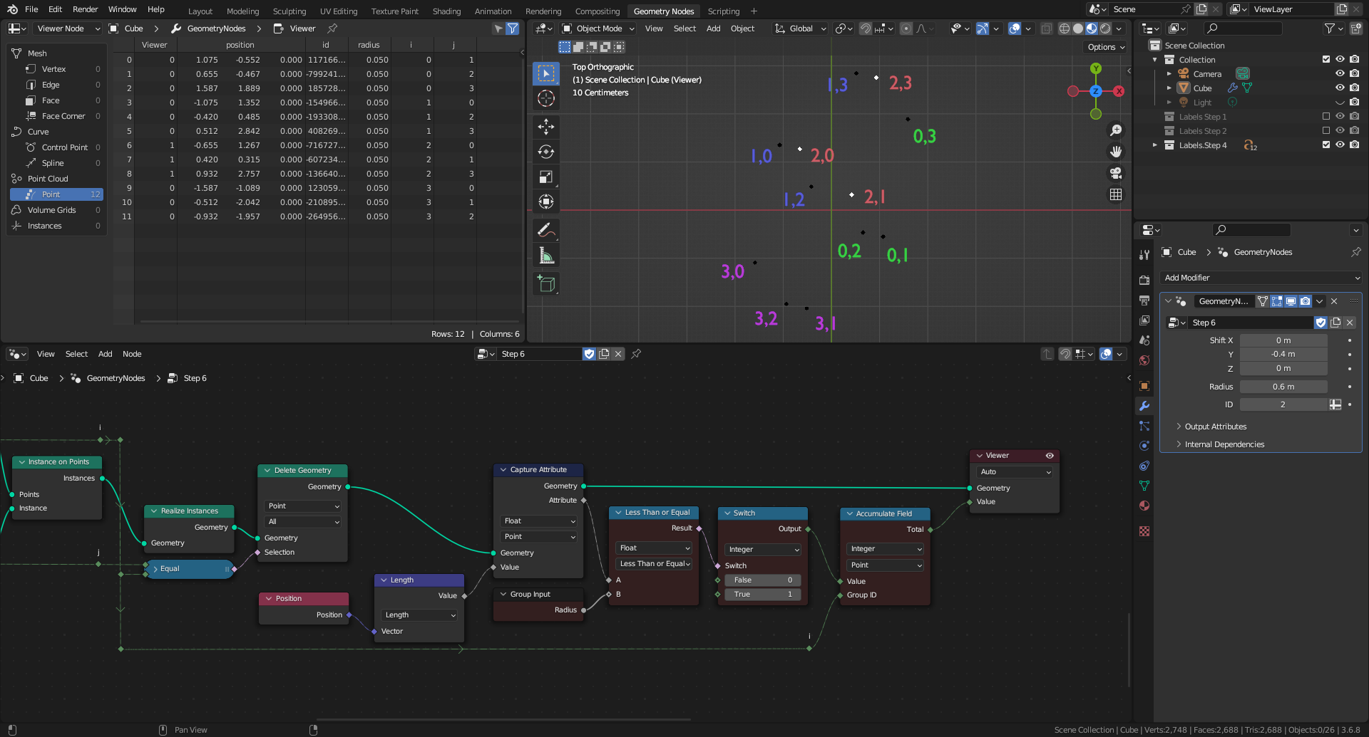
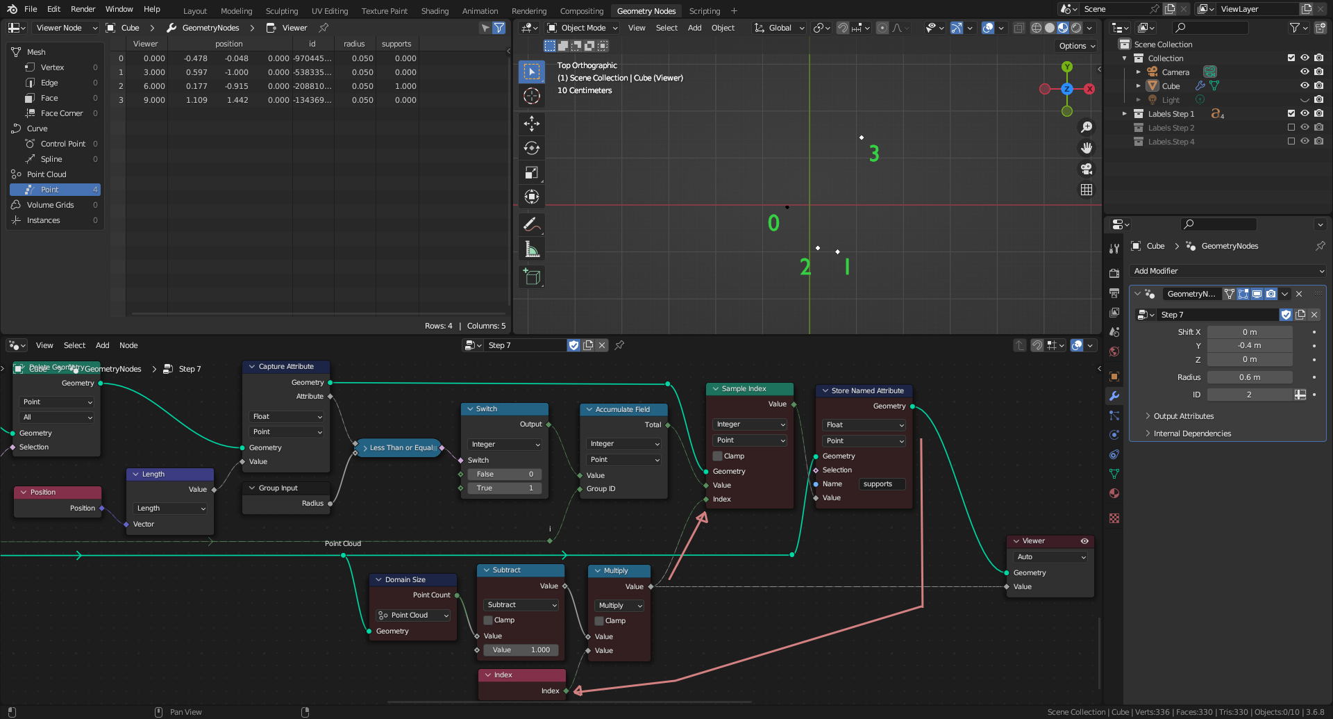
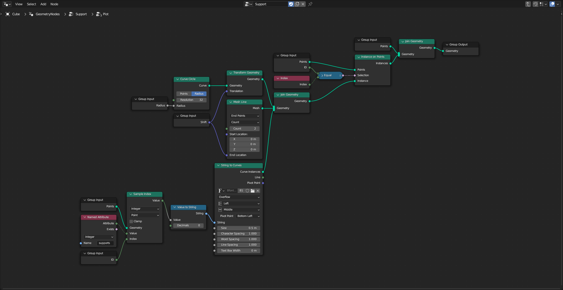
(Using Blender 3.6.8)

(NB: documentation to be continued...)

Acknowledgement: This proposal is adapted from the "quadratic geometry explosion" algorithm developed by Markus von Broady to solve "Compute on all points in geometry nodes". It takes also advantage of the test case introduced by Gordon Brinkmann in his proposal.

Objectives

Approach

GeometryNodes modifier

In what follows, the main graph is split in sequential parts that are discussed one at a time. To ease the display, previous parts might be off-window, and next parts are deleted. Nodes under discussion are in dark red. Extra nodes, not included in the main graph, are in dark green; these are added to display more information than required to perform efficiently the task.

Step 1

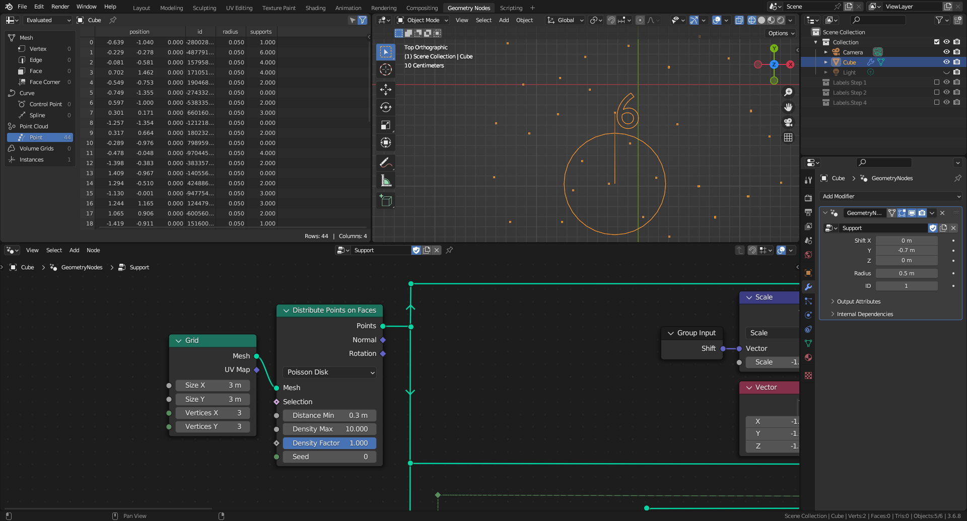
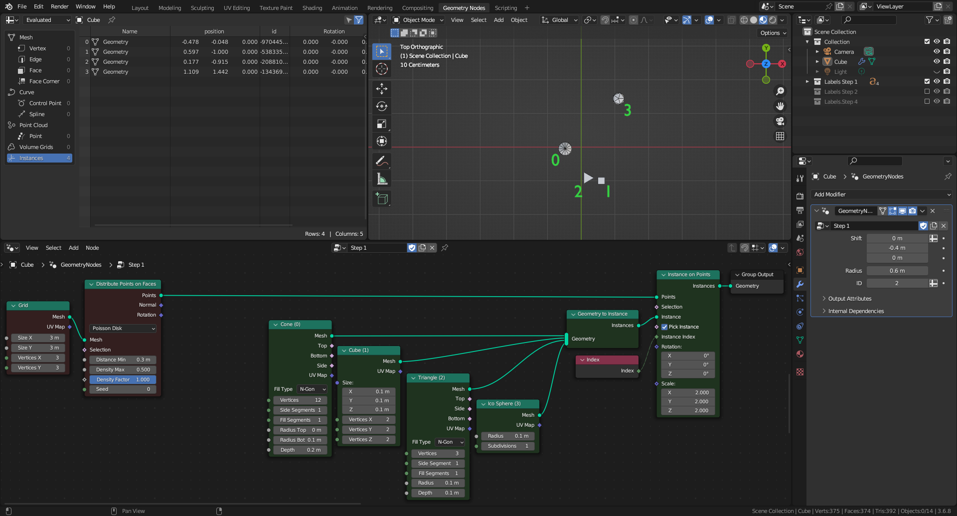
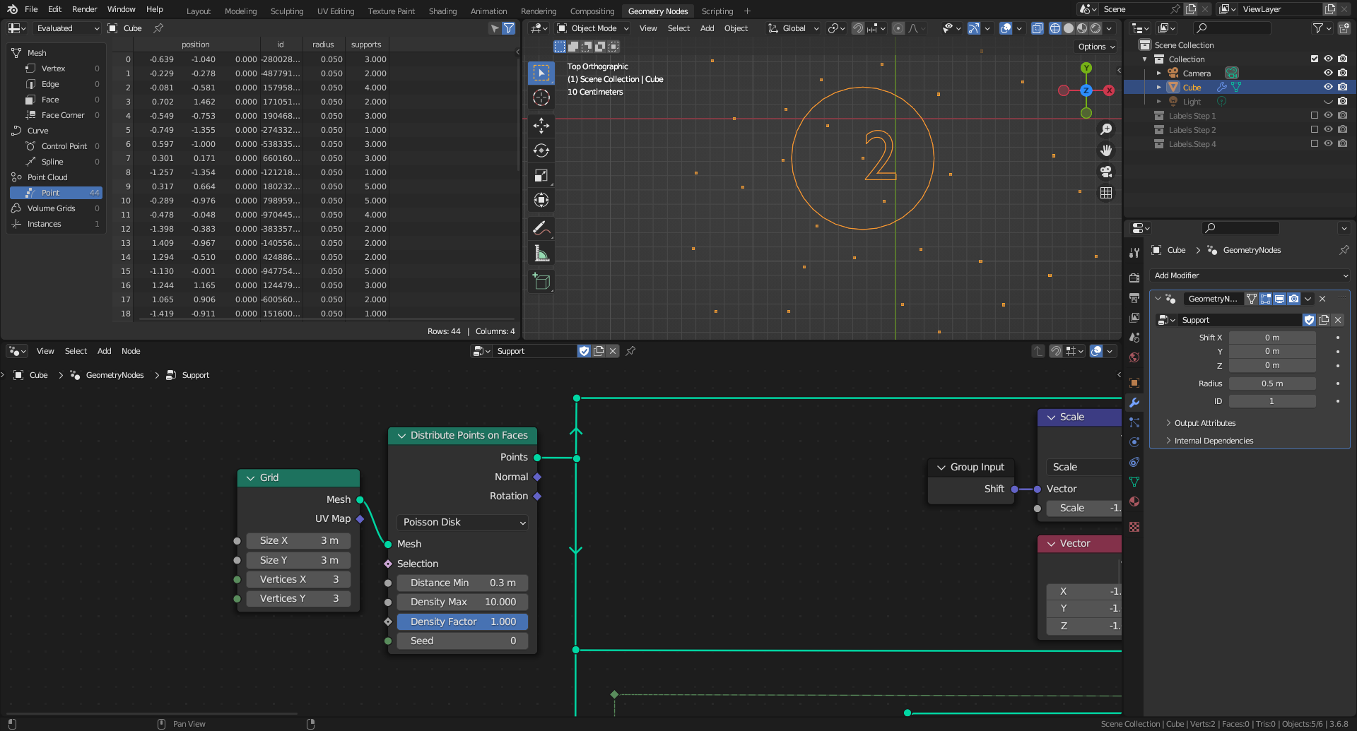
1. The 2D test case is based on a Grid node coupled to a Distribute Points on Faces node to create a Point Cloud. To limit the number of points to 4, the Density Max parameter is decreased from 10 to 0.5.
2. To visualise the Point Cloud, different mesh primitives are instanced on Points, ticking the Pick Instance parameter.
3. A Geometry to Instance node is used to make an ordered collection from a Cone, a Cube, a Cylinder (with 3 vertices, so a "Prism") and an Ico Sphere.
4. The Index of each point is added "by hand" through a collection of labels to be displayed in the 3D Viewport.

Step 2

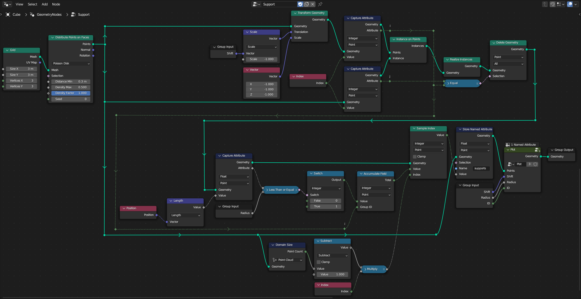
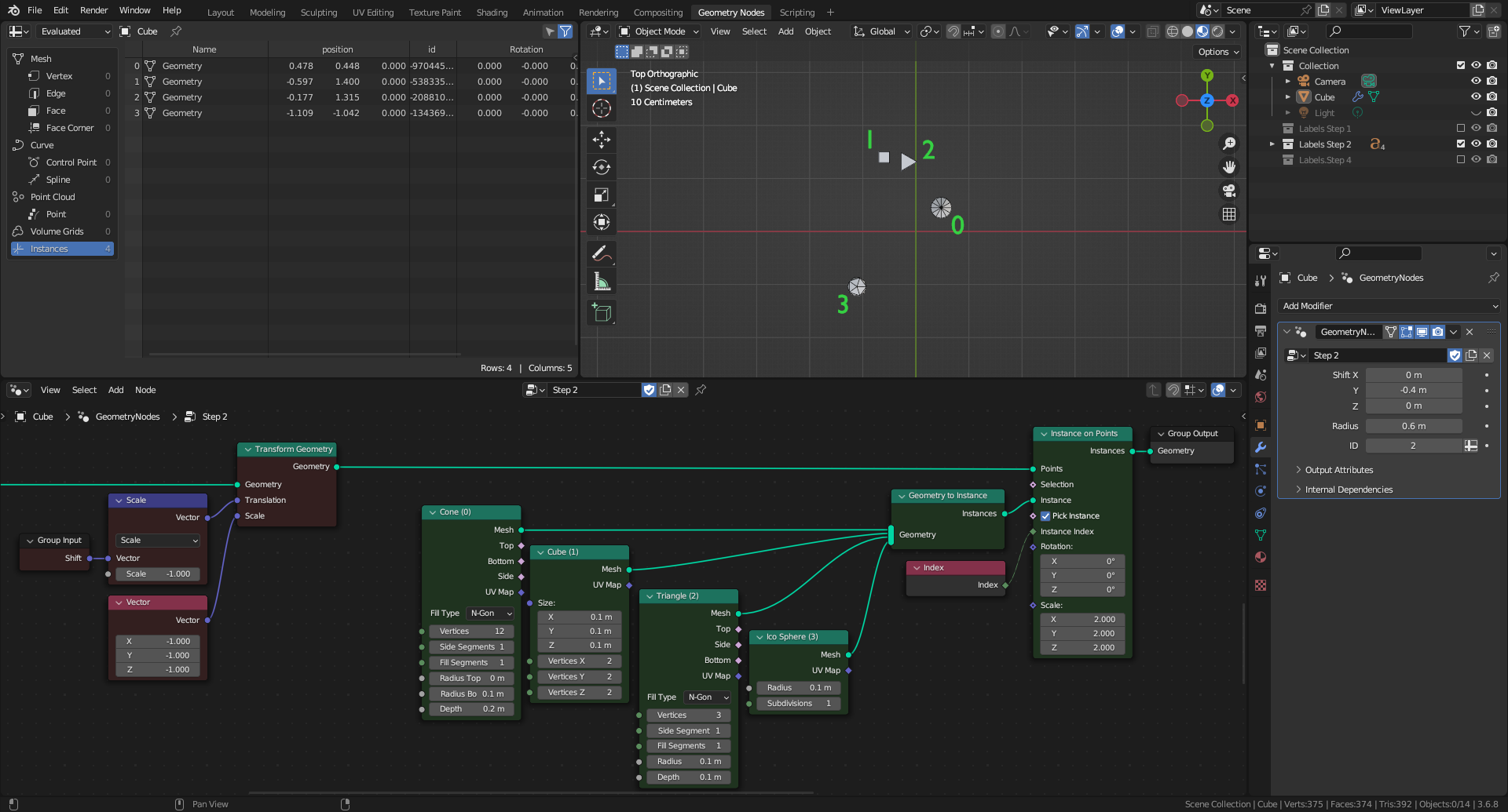
1. To compute the vector $\vec{x_j}-(\vec{x_i}+\vec{s})$, an occurrence of the original Point cloud is firstly transformed, such that new point coordinates are $\vec{x_{i}^{*}} = -\vec{x_i}-\vec{s}$, through a Transform Geometry node.
2. A component-wise Scaling by (-1,-1,-1) is used to compute $-\vec{x_i}$ from $\vec{x_i}$.
3. Because Translation is applied after Scaling, the Shift vector $\vec{s}$ is pre-multiplied by -1, to compute effectively $\vec{x_{i}^{*}} = -1 \times \vec{x_i}+(-1 \times \vec{s})$.
4. Consequently in the 3D Viewport, comparing Step 1 and Step 2 display, mesh primitives are moved by a symmetry about the origin, then by a translation opposite to $\vec{s}$ (i.e. upwards in the test case as $\vec{s}$ is set to -0.4 along the Y axis).

Step 3

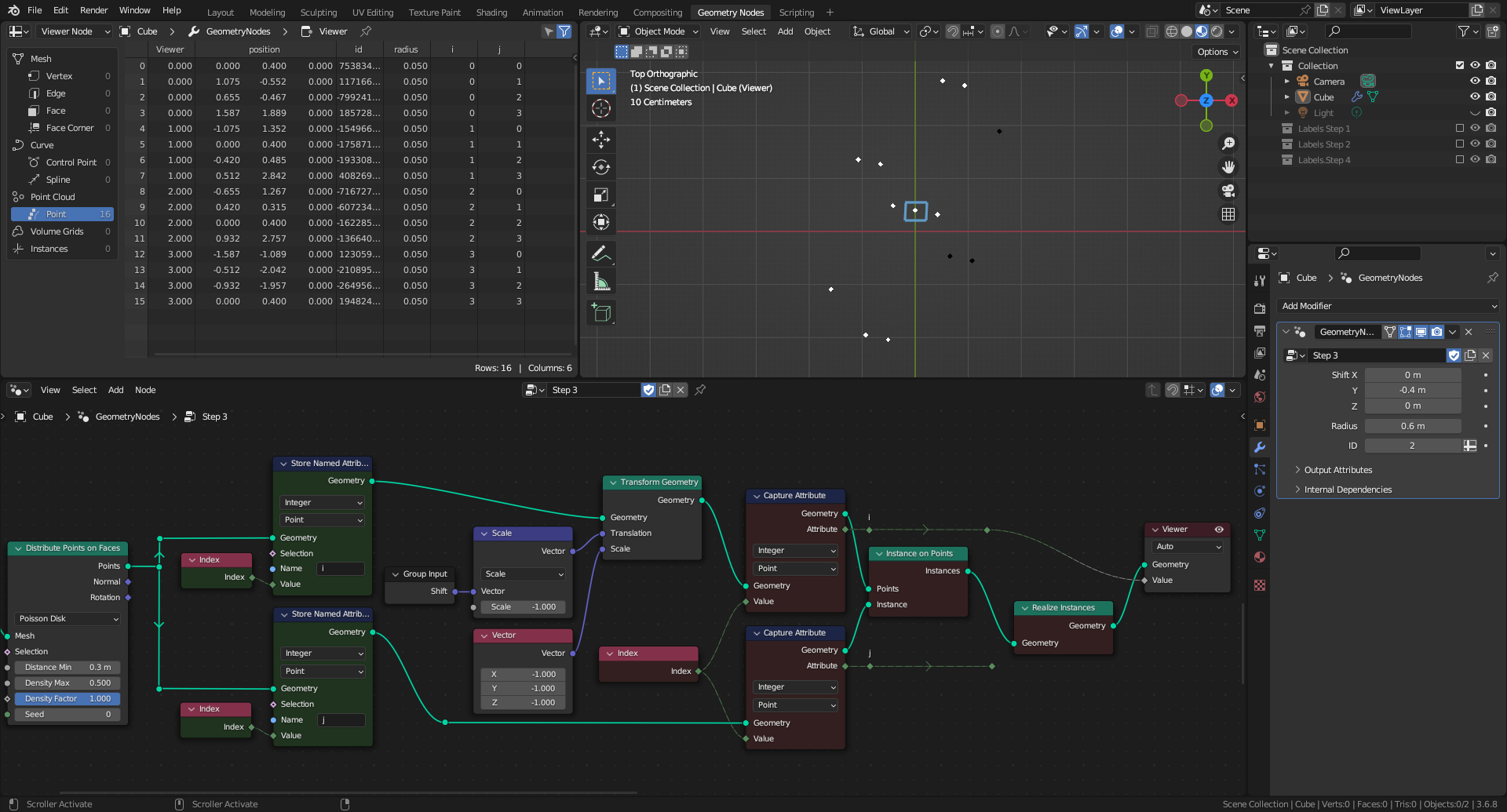
1. To create $N \times N \ (i,j)$ pairs, both input sockets of an Instance on Points node are connected to the same Point Cloud object, except that one occurrence was "symmetrized and shifted" at Step 2.
2. Index $i$ is arbitrarily associated to the Points socket, while index $j$ is associated to the Instance socket. Both are captured in Point domain for later usage before the Instance on Points node.
3. Vector $\vec{x_j}-(\vec{x_i}+\vec{s})$ is computed by a Realize Instances node as the instanced points position. Indeed this node is shifting the instanced objects position (i.e. $\vec{x_j}$) by the "instancer" point position (i.e. $\vec{x_{i}^{*}} = -(\vec{x_i}+\vec{s})$).
4. Consequently, 16 points are displayed in the Spreadsheet editor. To visualize simultaneously $i$ and $j$, these are transiently stored as Named Attributes explicitly. Viewer node is showing that captured and stored values are the same.
5. Side note: It is to notice that the building sequence of the Instance on Points node is running the "inner" loop on $j$ (column index) and the "outer" loop on $i$ (row index), i.e. as in a row-oriented table.
6. All $N \ (i,i)$ pairs are located at the same position (i.e. $-\vec{s}$) by construction. It is highlighted with a blue square in the 3D Viewport.

Step 4

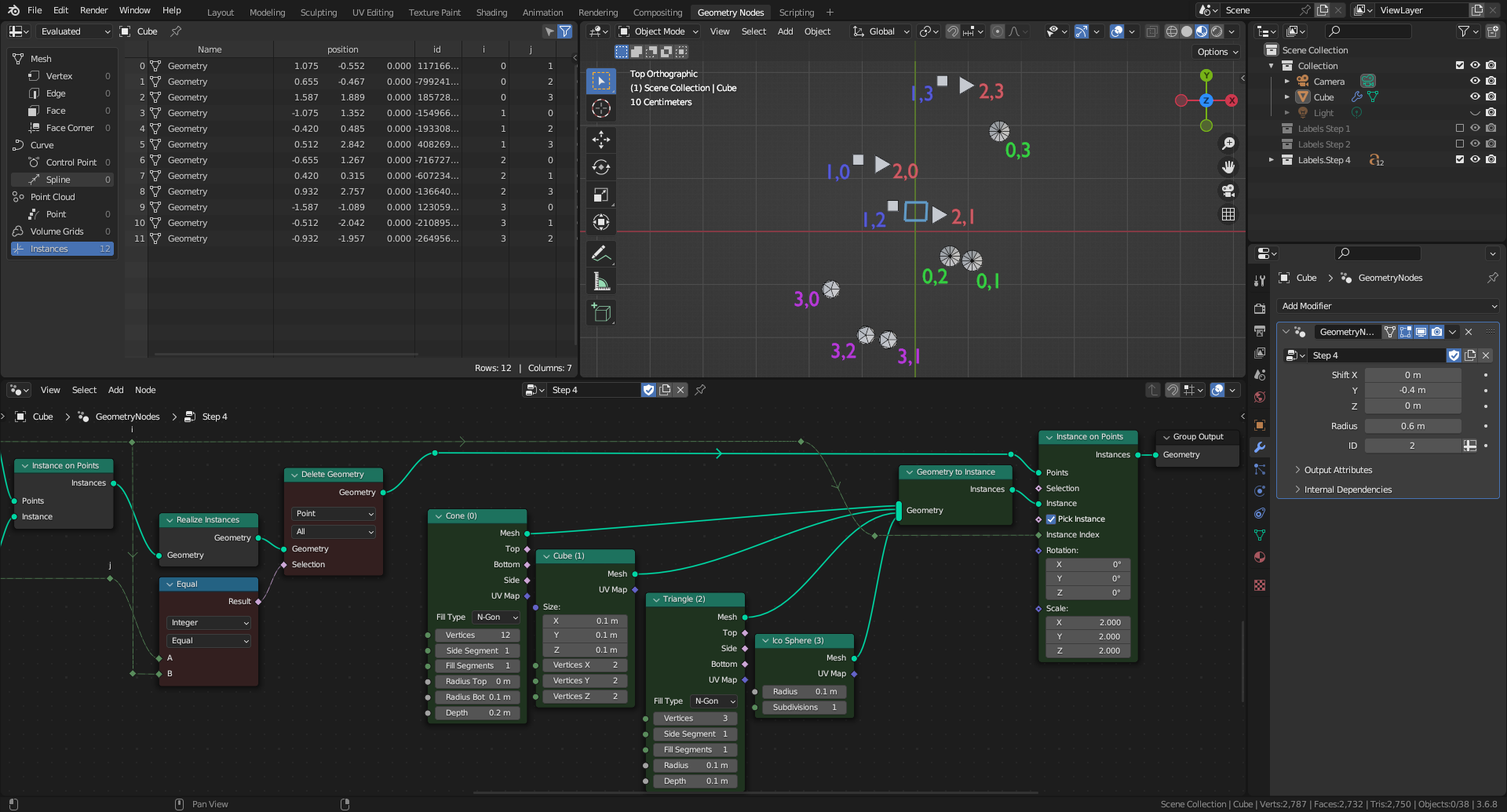
1. A Delete Geometry node set in Point domain is removing self-interactions, i.e. points such that $i=j$.
2. Consequently, only 12 points are remaining in the Spreadsheet editor, and the blue square is now empty in the 3D Viewport.
3. To visualise $(i,j)$ pairs position, the same object "$(i)$" as at Step 2 is instanced. Besides "$i,j$" value for each point is added "by hand" through a collection of labels.

Step 5

1..
2..
3..
4..
5..
6..
7..
8..
9..
10..

Step 6

1..
2..
3..
4..
5..
6..
7..
8..
9..
10..

Step 7

1..
2..
3..
4..
5..
6..
7..
8..
9..
10..

Stack Exchange Network

How to calculate an attribute for each point which depends on every other point