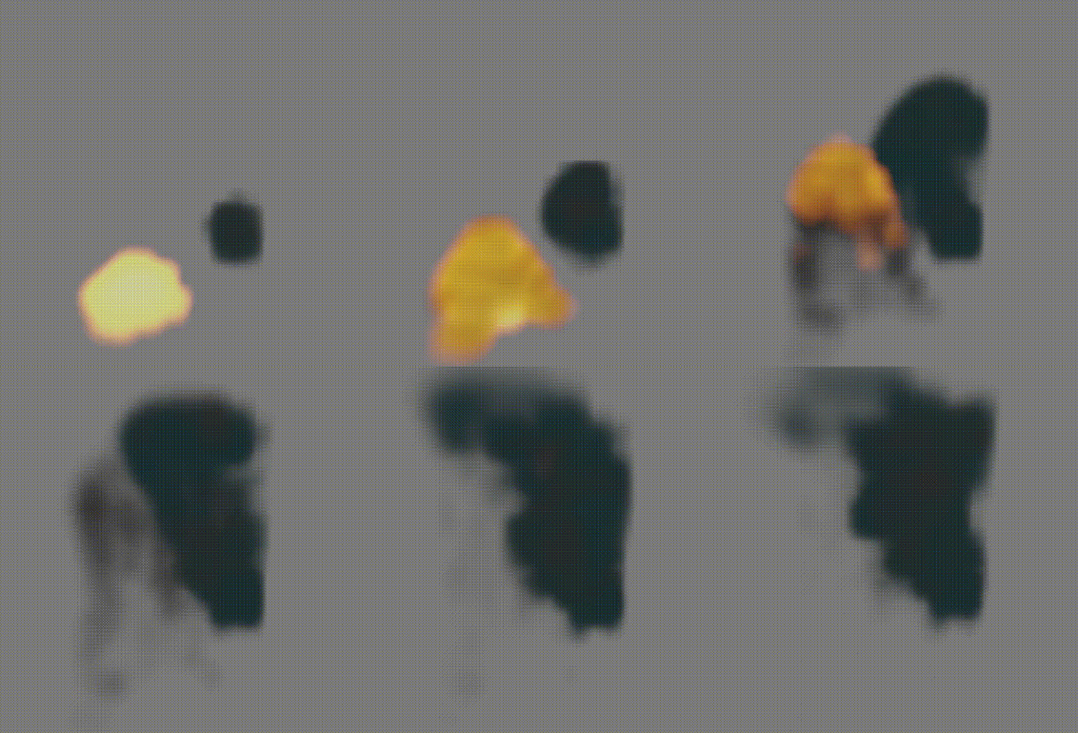
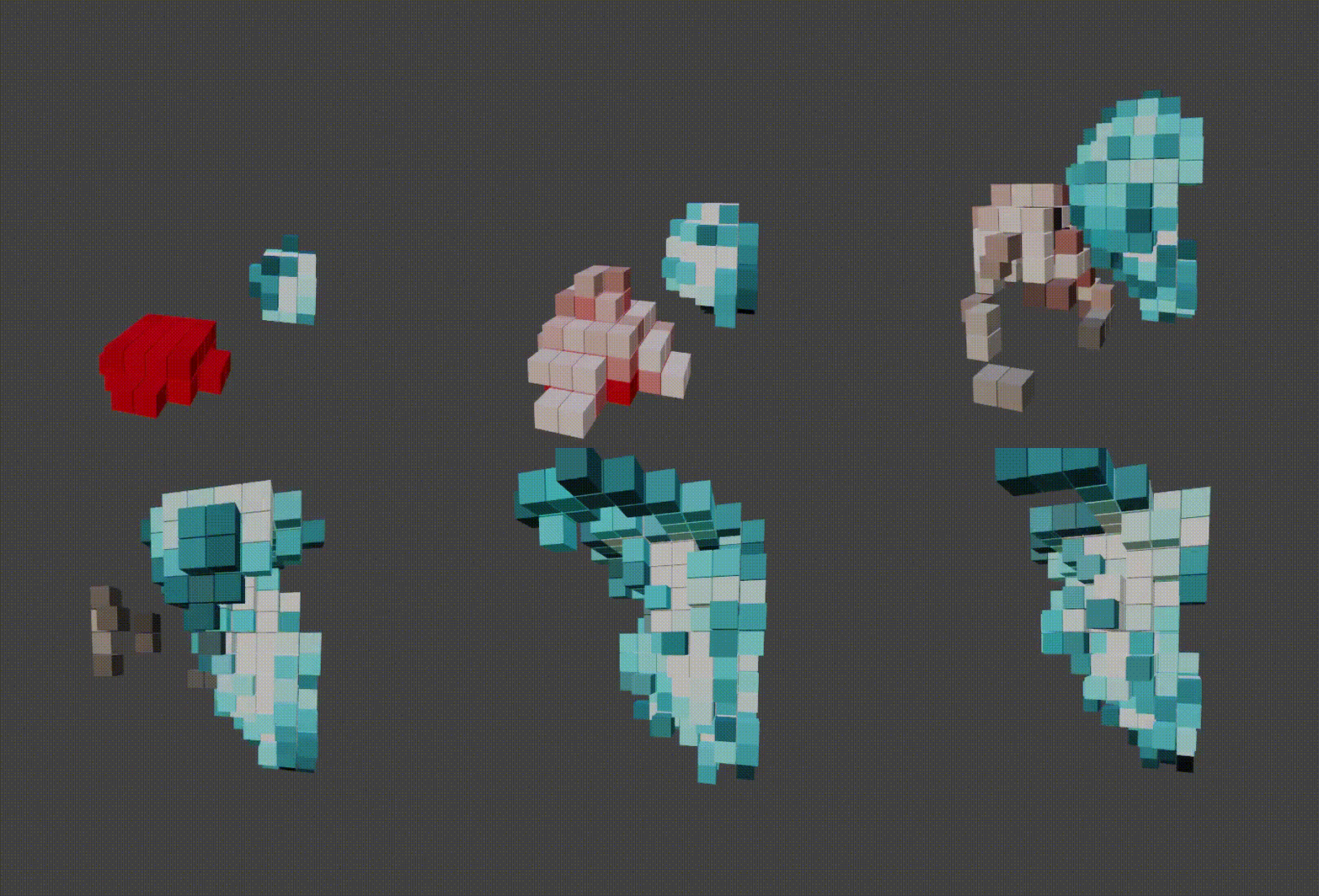
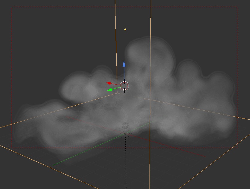
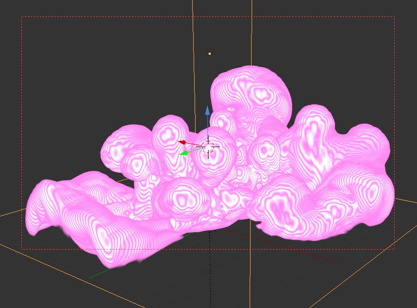
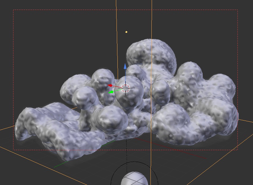
For python coders, I will add an answer demonstrating the python access to the smoke system.
The simulated smoke is stored in the modifier.
- Access the correct modifier of the smoke domain object.
- Go to its
domain_settings.
- The data is stored in a uniform grid, the resolution sets the divisions for the longest dimension.
- It has the properties
density_grid, flame_grid, color_grid. The first two are flat lists, which you can arange in an zyx grid. The color_grid has an additional dimension for rgba values.
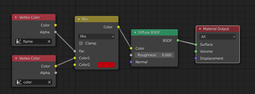
I would suggest storing these values in vertex colors.
For further processing I would suggest the remesh modifier and the color transfer using Animation Nodes.


Example Usage
You can grab the script (also included in the blend) from github. To use the script you have to setup your file first, as the script makes assumptions about the existence of some object.
- Create a cube-shaped (equal dimensions!) domain object and name it domain.
- Add other inflow/outflow/obstacle objects and bake the simulation.
- Create a collection named simulated. For our convenience, the script will place the created geometry there.
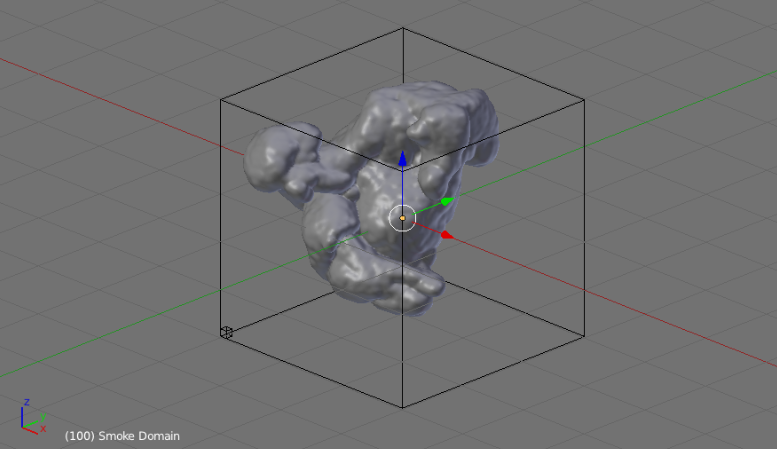
- Open a Text Editor in a Blender area and copy-paste the script into a new textblock. With the script textblock open, go to the text editors menu and selected Text > Run Script. If the script runs correctly, mesh objects are placed in the simulated collection.

Running the script in the example file will immediately crash Blender if you haven't baked the simulation yet.
Follow these steps to test the example file.
- Go into solid viewport mode. Unhide the Collection and select the smoke domain object.
- Rebake the simulation under Physics Properties > Fluid (Domain) > Settings > Free Data + Bake.
- Open the console for logging.
- Run the script via Text > Run Script. When running the script, both collections have to be active and visible and the smoke simulation cached.
Step By Step Explanation
The first step of a python script is to import so-called modules. These modules provide functionality, which python can access. The bpy module contains functionality to access Blenders data. bmesh is a representation of mesh objects. numpy is a library to manipulate numbers and in ours case matrices. The result of the smoke simulation is stored in a grid, which numpy can easily manipulate.
import bpy
import bmesh
import numpy as np
import mathutils
Next, I add a utility function. This functions receives a string name as a parameter and returns an object of that name. If the object doesn't exist yet, it creates a new mesh-object. If it exists it returns the same mesh object. With this helper function we can run the meshing function multiple times and simply overwrite our created objects without creating additional object.001 each time.
def get_mesh(name):
    if bpy.data.objects.get(name) == None:
        me = bpy.data.meshes.new(name)
        bpy.data.objects.new( name, me )
    return bpy.data.objects[name]
Now come the main method, which gets the smoke simulation and accesses its properties on the current frame. The result gets written into a bmesh (Blenders module for mesh representation and manipulation).
The function definition start with def in python.
def write_smoke_to_bm(smoke_obj, bm):
I'm assuming that the smoke modifier is the first (with the index 0) modifier in the modifier stack modifiers. If it wasn't the index has to be adjusted. The modifiers has a property called domain_settings, which contains the domain settings of the smoke simulation.
    smoke_domain_mod = smoke_obj.modifiers[0]
    settings = smoke_domain_mod.domain_settings
The domain_settings object has the properties resolution_max, density_grid, color_grid and flame_grid. The first is simply the grid resolution which we set in the domain settings. We need to know this, because the voxel data is stored in a grid with this resolution. To simplify the matter, I restricted the domain object to uniform dimensions (as mentioned earlier) which result in a three-dimensional grid with resolution_max slots for each axis (x, y, z). The other objects are data object in the form of the grid. However, this data is stored in a long list, which we have to manually convert to a grid form. Converting it is optional, but very helpful. It is much more convenient to access the grid position with x, y, z coordinates instead of the nth position in a long list. This is were the numpy library comes in handy, because it can "reshape" the list into a 3 dimensional list. The density_grid and flame_grid are simply three dimensional grid now with a number representing the amount of density/flame.
Since we only want to add geometry where the density is high enough, I defined a density threshold (thres), which is a fourth of the highest density value in the whole grid.
    res = settings.resolution_max
    grid_density = np.array(settings.density_grid).reshape((res, res, res))
    grid_col = np.array(settings.color_grid).reshape((res, res, res, 4))
    grid_flame = np.array(settings.flame_grid).reshape((res, res, res))
    thres = np.max(grid_density)/4
Now, we construct a bounding box of the dimensions. Using numpy again, we can story the values of all the vertices of the smoke object (smoke_obj) in a matrix and extract the smallest and highest values of the vertices' coordinates for each of their axes. The variable minmax stores them as [[x_min, y_min, z_min], [x_max, y_max, z_max]].
In the same manner, we can calculated the step size of a single voxel. Since the number of steps is defined by the resolution_max, the size of the voxel (along the x axis for example) can be defined as (x_max - x_min) / resolution_max.
    verts = np.array([smoke_obj.matrix_world @ v.co for v in smoke_obj.data.vertices])
    verts = verts.reshape((*verts.shape, 1))
    minmax = np.stack((np.min(verts, axis=0), np.max(verts, axis=0)))
    minmax = np.reshape(minmax, minmax.shape[:2])

    step = (minmax[1] - minmax[0]) / res
The bmesh object, which we passed as a parameter to the function, story vertex colors in loops, which are the vertices of a single face. Since the vertex color layers probably don't exist, we can create them.
    density = bm.loops.layers.color.new("density")
    color = bm.loops.layers.color.new("color")
    flame = bm.loops.layers.color.new("flame")
In the next step we loop through the slot of the three-dimensional density grid (or numpy-matrix).
    for z in range(0, grid_density.shape[0]):
        for y in range(0, grid_density.shape[1]):
            for x in range(0, grid_density.shape[2]):
Then we check if this position in the grid is dense enough to "mesh" it. We use the threshold, which we defined earlier.
if grid_density[z, y, x] > thres:
If it is dense enough, we can place a cube there. Or a sphere, or a single face or anything else. I use a cube, because there is a simple builtin function in the bmesh module: create_cube.
To properly position this cube, we have to supply it with the translation and scale in form of a matrix. Blenders mathutils method provides functions which can generate a matrix from translation and scale values.
                    mat = mathutils.Matrix.Translation((
                        minmax[0][0] + (x + 0.5) * step[0],
                        minmax[0][1] + (y + 0.5) * step[1],
                        minmax[0][2] + (z + 0.5) * step[2]
                    )).to_4x4()
                    mat = mat @ mathutils.Matrix.Diagonal(step * 0.95).to_4x4()

                    verts = bmesh.ops.create_cube(bm, size=1, matrix=mat)['verts']
The create_cube function returns a dictionary object with an entry for the created vertices. Let's get the linked faces of those vertices.
                    faces = set()
                    for v in verts:
                        for face in v.link_faces:
                            faces.add(face)
Once we have the faces, we get the linked loops (think face corners) and assign their vertex-color layers (which we created earlier) the respective values. The density layer gets the density value, the color layer gets the color value and the flame layer gets the flame value. In the cases of the color layer we can simply assign the color rgba values at that slot to the loop. But in the cases of the density and flame we only have one value. That's why we use the python syntax of [density_value] * 4 to create an rgba value as well to store in the vertex color layer: e.g. 1.2 => [1.2, 1.2, 1.2, 1.2].
                    for face in faces:
                        for loop in face.loops:
                            loop[density] = [grid_density[z, y, x]] * 4
                            loop[color] = grid_col[z, y, x]
                            loop[flame] = [grid_flame[z, y, x]] * 4
This is the end of the function, which adds the geometry to a bmesh.
Now you can loop over all of the frames and create an object with the previous function.
Since we will have to do this for each frame individually, I will first gather a list of frames. The list of frames is defined by the cache start and end of the smoke domain object.
domain = bpy.data.objects['domain']
smoke = domain.modifiers[0]

depsgraph = bpy.context.evaluated_depsgraph_get()
smoke_obj = domain.evaluated_get(depsgraph)
smoke_domain_mod = smoke_obj.modifiers[0]
settings = smoke_domain_mod.domain_settings
Just as before, this was the same code to get to the smoke domain settings, which store the properties cache_frame_start and cache_frame_end.
To organize our Blender file, the created objects are best placed in their own collection: simulated. Let's get a reference to that as well.
objects = bpy.data.collections['simulated'].objects
Now we can loop through all the frames. Since Blender becomes unresponsive for the duration of the execution of a python script, it is helpful to open the blender console (Window > Open Console) and print the current frames, which Blender is working on. frame_set advances the scene to a given frame and updates the objects and the smoke simulation state.
for frame in range(settings.cache_frame_start, settings.cache_frame_end):
    print(frame)
    bpy.context.scene.frame_set(frame)
Get the current smoke simulation frame with the evaluated dependency graph.
    depsgraph = bpy.context.evaluated_depsgraph_get()
    smoke_obj = domain.evaluated_get(depsgraph)
Create a new bmesh to hold the smoke mesh data for this frame. Then pass it to the function, which we wrote ealier.
    bm = bmesh.new()
    write_smoke_to_bm(smoke_obj, bm)
Using the helper function (also from above), we can create/get an object named simulated##, where ## stands for the current frame number. We write the bmesh data into that objects mesh and free the bmesh.
    ob = get_mesh('simulated' + str(frame).zfill(2))
    bm.to_mesh(ob.data)
    bm.free()
If the frame mesh object didn't exist, it would have been created. For that case, we have to move it into the simulated collections objects "list".
    try:
        objects.link(ob)
    except:
        pass # already in collection
If you were to execute the code uptill now, all mesh objects would be created and visible at once. This could be useful if you want to modify them further, etc. If you want to judge the playback however, you would rather only see the mesh object, which corresponds to the current frame. To achieve this, you can keyframe the visibility property of objects with the function keyframe_insert.
    for i in (frame - 1, frame + 1):
        ob.hide_viewport = ob.hide_render = True
        ob.keyframe_insert('hide_viewport', frame=i)
        ob.keyframe_insert('hide_render', frame=i)
    ob.hide_viewport = ob.hide_render = False
    ob.keyframe_insert('hide_viewport', frame=frame)
    ob.keyframe_insert('hide_render', frame=frame)
If you want to see any colors, set the viewport to vertex color mode or link the objects to a material, which uses the vertex colors we created.
