Under work...
(Using Blender 3.6.5 and Geometry Nodes)
Objectives
| Requirements |
To achieve |
1 - Animate a sine wave:
- of constant amplitude,
- with a smooth transition between two wavelengths.
2 - Use it as a Driver.
3 - Bonus: Use the Graph Editor to control the transition. |

|
Documentation
Preliminary remarks
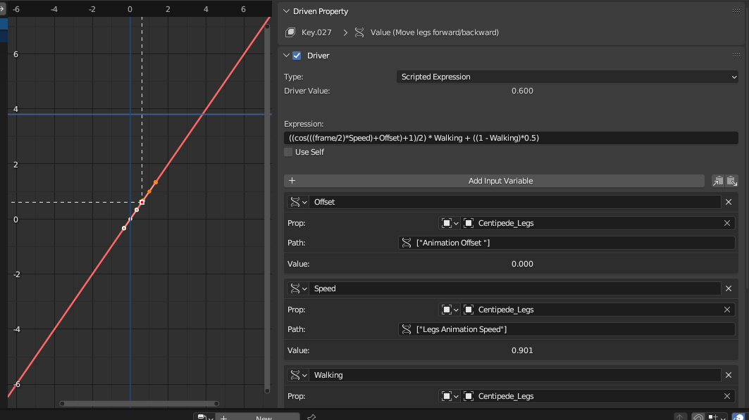
Stripped of extra parenthesis and assuming $\textrm{Walking}=1$, the recast expression reads:
$$f(\textrm{frame}) = \frac{1}{2} \left\{ \cos{\left( \frac{1}{2} \times \textrm{frame} \times \textrm{Speed} + \textrm{Offset} \right)} + 1 \right\} \label{eq_f_Frame} \tag{1}$$
So $\textrm{Speed}$ is homogenous to radian per frame.
Defining the time $t=\textrm{frame}$ in frames, the angular frequency $\omega=\frac{1}{2} \textrm{Speed}$ in radian per frame and the phase shift $\varphi=\textrm{Offset}$ in radian, Equation (\ref{eq_f_Frame}) is written:
$$f(t) = \frac{1}{2} \left\{ \cos{\left(\omega t+ \varphi \right)} + 1 \right\} \label{eq_f_t} \tag{2}$$
Defining the phase $\theta=\omega t+ \varphi$ in radian, Equation (\ref{eq_f_t}) is written:
$$f(\theta) = \frac{1}{2} \left\{ \cos{\theta} + 1 \right\} \label{eq_f_theta} \tag{3}$$
So for an infinitesimal variation of $\theta$, the variation of $f$ is:
$$df = -\frac{1}{2} \sin{\theta} \ d\theta \label{eq_df} \tag{4}$$
Mathematical analysis
Regularity of $f$ and $df$
From Equation ($\ref{eq_f_theta}$), $f$ is continuous if $\theta$ is continuous. From equation ($\ref{eq_df}$), the variation of $f$ is smooth if $d \theta$ is continuous.
It is to notice that:
$$ d\theta = \omega dt + t d\omega + d\varphi \label{eq_dtheta_phi} \tag{5}$$
Assuming that $\varphi(t)$ is a constant piecewise function yields $d\varphi=0$ and:
$$d\theta = \omega dt + t d\omega \label{eq_dtheta_dt} \tag{6}$$
So $d\theta$ is continuous even if $\omega(t)$ is discontinuous as long as the right-hand side of Equation ($\ref{eq_dtheta_dt}$) is continuous, meaning that $d\omega$ is discontinuous too.
Relation between time and phase
Let introduce $T(t)$ such that:
$$ \frac{T}{dt} = \frac{2\pi}{d\theta} \label{eq_T} \tag{7}$$
If $T$ were constant and $dt$ were assimilated to a constant time step, $d\theta$ would be constant too. The left-hand side would be the number of frames required to span one cycle, while the right-hand side would be the number of angular samples required to span one cycle.
So $T$ is the apparent number of frames per cycle at time $t$.
Rewriting Equation ($\ref{eq_T}$) as:
$$ \frac{d\theta}{2\pi} = \frac{dt}{T} \label{eq_dtheta} \tag{8}$$
states that between two adjacent frames, the fraction of a round in phase is equal to the fraction of a period in time.
General formulation of $\theta(t)$
As a conclusion, $T(t)$ is the wavelength in frames, same as the period in time, that is assumed to vary continuously.
By integration of $d\theta$ from Equation ($\ref{eq_dtheta}$), defining $\theta_0$ as the phase at $t=0$, the general expression of $\theta(t)$ is:
$$\theta(t) = \theta_0 + 2 \pi \int_{0}^{t} \frac{d\tau}{T(\tau)} \label{eq_theta_integral} \tag{9}$$
Equation ($\ref{eq_theta_integral}$) combined with the continuity of $T(t)$ guaranties that $\theta$ and $d\theta$ are continuous.
Analytical solutions for $\omega(t)$ and $\varphi(t)$
Given the analytical expression of $T(t)$, Equation ($\ref{eq_theta_integral}$) yields $\theta(t)$, then $\omega(t)$ and $\varphi(t)$.
Let $t_L$ and $t_R$ be two times such that $t_L < t_R$. Let $T_L$ (resp. $T_R$) be the period for $t \leq t_L$ (resp. for $t \geq t_R)$. So:
$$ \left\{ {\begin{array}{llll}
\forall t, t \leq t_L, &
\omega(t)=\omega_L=\frac{2 \pi}{T_L}, &
d\omega = 0, &
d\theta = \omega_L dt \\
\forall t, t \geq t_R, &
\omega(t)=\omega_R=\frac{2 \pi}{T_R}, &
d\omega = 0, &
d\theta = \omega_R dt
\end{array}}
\right. \label{eq_T_L_T_R} \tag{10}$$
In what follows, upper-script $[]^{-}$ means the limit by lower value of $t$, while upper-script $[]^{+}$ means the limit by higher value of $t$.
Expression of $\varphi(t)$
Assuming that the phase shift $\varphi_L^{-}$ is know and constant for $t \leq t_L$, the continuity of $\theta$ for $t=t_L$ leads to:
$$ {\begin{array}{lrcl}
\mbox{} & \theta(t_L^{-}) & = & \theta(t_L^{+}) \\
\Leftrightarrow &
\omega(t_L^{-}) \ t_L + \varphi_L^{-} & = &
\omega(t_L^{+}) \ t_L + \varphi_L^{+} \\
\Leftrightarrow &
\varphi_L^{+} & = & \varphi_L^{-} + \left[
\omega_L - \omega(t_L^{+}) \right] \ t_L
\end{array}}\tag{11}$$
While the continuity of $\theta$ for $t=t_R$ leads to:
$$ \varphi_R^{+} = \varphi_R^{-} + \left[ \omega(t_R^{-}) - \omega_R \right] \ t_R \label{eq_phi_R} \tag{12}$$
It is to notice that if $\omega$ is not continuous at $t=t_L$ or $t=t_R$, $\varphi$ is discontinuous too.
So whatever the expression of $\omega(t)$ for $t_L \lt t \lt t_R$ is, the phase shift $\varphi(t)$ is defined by:
$$\left\{ {\begin{array}{llll}
\forall t, t \leq t_L, &
\varphi(t)= \varphi_L^{-} \\
\forall t, t_L \lt t \lt t_R, &
\varphi(t)= \varphi_L^{+} = \varphi_R^{-} \\
\forall t, t \geq t_R, &
\varphi(t)= \varphi_R^{+} \\
\end{array}}
\right. \label{eq_phi_t} \tag{13}$$
Case: Step variation of $T(t)$
Assuming that $t_L=t_R=t_{LR}$ leads to the Heaviside step function for $\omega(t)$. $\theta(t)$ is continuous at $t=t_{LR}$, but $d\theta$ is not because $d\theta^{-}=\omega_L dt$ while $d\theta^{+}=\omega_R dt$.
$\omega(t)$ and $\varphi(t)$ are defined by:
$$ \left\{ {\begin{array}{lll}
\forall t, t \lt t_{LR}, &
\omega(t)=\omega_L, &
\varphi(t) = \theta_0 \\
\forall t, t \gt t_{LR}, &
\omega(t)=\omega_R, &
\varphi(t) = \theta_0 + \left[
\omega_L - \omega_R \right] \ t_{LR}
\end{array}}
\right. \label{eq_Heaviside} \tag{14}$$
This is illustrated in the next figure with $\theta_0=0$, where the switch between $T_L$ yielding 25 frames per period and $T_R$ yielding 50 frames per period is triggered between frames $t_L=59$ and $t_R=60$ (indicated with purple vertical lines). In the top sub-figure, $f(t)$ is drawn with blue plus signs and $T(t)$ with red solid line. $f(t)$ is continuous, but as expected, the period is not. In the bottom sub-figure, $d\theta$ normalised by $\omega_L dt$ is plotted with red dotted line, to compare to $\omega(t)$ in blue solid line. As expected, it is equal to $\omega_L dt$ for $t \lt t_L$, and to $\omega_R dt$ for $t \gt t_R$, with a discontinuity between. $\varphi(t)$ in green solid line is also discontinuous.

Case: Linear variation of $T(t)$
Assuming that for $t_L \lt t \lt t_R$, $T(t)=a_0+a_1 \ t$, and that for $t \leq t_L$, $\varphi(t) = \theta_0$, Equation ($\ref{eq_theta_integral}$) reads:
$$\theta(t) = \theta_0 + 2 \pi \int_{0}^{t_L} \frac{d\tau}{T_L} + 2 \pi \int_{t_L}^{t} \frac{d\tau}{a_0+a_1 \tau} \label{eq_theta_integral_Linear} \tag{15}$$
It leads to:
$$\theta(t) = \theta_0 + \omega_L \ t_L + \frac{2 \pi}{a_1} \ln{ \left[ \frac{a_1}{T_L} (t-t_L) + 1 \right]} \label{eq_theta_Linear} \tag{16}$$
So for $t_L \lt t \lt t_R$, $\omega(t)$ and $\varphi(t)$ are defined by:
$$ \left\{ {\begin{array}{lcl}
\omega(t) & = & \frac{1}{t} \frac{2 \pi}{a_1} \ln{ \left[ \frac{a_1}{T_L} (t-t_L) + 1 \right]} \\
\varphi(t) & = & \theta_0 + \omega_L \ t_L
\end{array}}
\right. \label{eq_omega_phi_linear} \tag{17}$$
It is to notice that $\omega(t_L^{+})=0$, so $\omega(t)$ is discontinuous.
$a_1$ is defined as:
$$ a_1 = \frac{t_L - t_R}{T_L - T_R} \label{eq_a1} \tag{18}$$
This is illustrated in the next figure, where the linear transition between $T_L$ yielding 25 frames per period and $T_R$ yielding 50 frames per period is occurring between frames $t_L=59$ and $t_R=250$. In the top sub-figure, $f(t)$ in blue and $T(t)$ in red are continuous. In the bottom sub-figure, $d\theta$ in red is continuous too, while $\omega(t)$ in blue and $\varphi(t)$ in green are not. It is to notice the log-shape of $\omega(t)$ for $t \in [t_L, t_R]$, and the discontinuity of its derivative at $t=t_L$ and $t=t_R$.

Implementation
Tool box
Computation of $f(\theta)$

This graph computes $f(\theta)$ following Equation ($\ref{eq_f_theta}$):
$$f(\theta) = \frac{1}{2} \left\{ \cos{\theta} + 1 \right\}$$
Computation of $\theta(t)$ from $T(t)$ controlled by the Graph Editor

This graph computes $\theta(t)$ by discretization of Equation ($\ref{eq_theta_integral}$):
$$\theta(t) = \theta_0 + 2 \pi \int_{0}^{t} \frac{d\tau}{T(\tau)}$$
as the accumulation inside a Simulation Zone of:
$$ \theta^{n+1} = \theta^{n} + d\theta^{n} \ \mathrm{with} \ d\theta^{n}=\frac{2 \pi}{T^{n}}$$
assuming that the animation of the Graph Editor is providing $T^n$ at frame $n$ and that the increment $d\tau$ between two adjacent frames is equal to 1.
1. The Simulation Input node provides $\theta^n$ and $d\theta^n$.
2. $\theta^{n+1}$ is computed from $\theta^{n}$ and $d\theta^{n}$.
3. $d\theta^{n+1}$ is computed from $T^{n+1}$.
4. $\theta^{n+1}$ and $d\theta^{n+1}$ are stored in the Simulation Output node.
5. At initialization, $\theta^{-1}=\theta_0$ and $d\theta^{-1}=0$ are input such that $\theta^0=\theta_0$.
6. To limit truncation errors, $\theta$ is kept in the interval $[0, 2 \pi]$.
Computation of $\theta(t)$ for the step variation of $T(t)$
 This graph computes $\theta(t)$ from $\omega(t)$ and $\varphi(t)$ at frame $n$.
1. $\omega_L$ and $\omega_R$ are computed from Equation ($\ref{eq_T_L_T_R}$).
2. $\omega^n$ and $\varphi^n$ are computed from Equation ($\ref{eq_Heaviside}$).
3. $\theta^n$ is computed as $\theta^n = \omega^n t^n + \varphi^n$.
Computation of $\theta(t)$ for the linear variation of $T(t)$
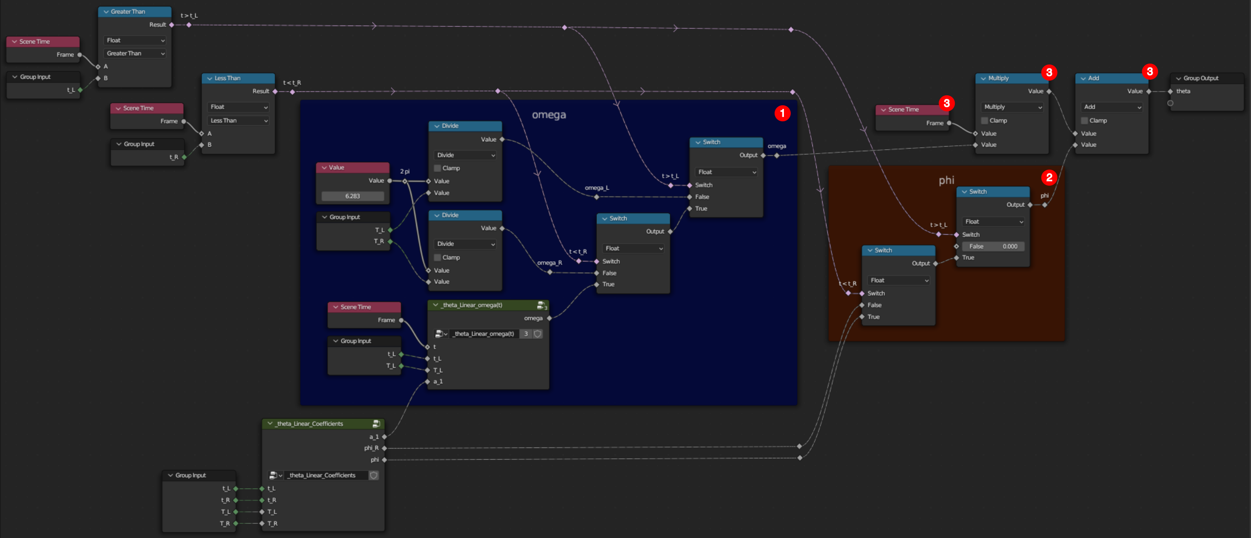
This part is divided into 3 groups.
 This graph computes $\omega(t)$ following Equation ($\ref{eq_omega_phi_linear}$):
$$ \omega(t) = \frac{2 \pi}{a_1 t} \ln{ \left[ \frac{a_1}{T_L} (t-t_L) + 1 \right]} $$
 This graph computes various constant coefficients.
1. $a_1$ is computed from Equation ($\ref{eq_a1}$).
1. $\varphi(t_L^+)=\varphi(t_R^-)$ is computed from Equation ($\ref{eq_omega_phi_linear}$).
1. $\varphi(t_R^+)$ is computed from Equation ($\ref{eq_phi_R}$).
 This graph computes $\theta(t)$ from $\omega(t)$ and $\varphi(t)$ at frame $n$.
1. $\omega_L$ and $\omega_R$ are computed from Equation ($\ref{eq_T_L_T_R}$), and $\omega(t)$ from Equation ($\ref{eq_omega_phi_linear}$), to determine $\omega^n$.
2. $\varphi^n$ is computed from Equation ($\ref{eq_phi_t}$).
3. $\theta^n$ is computed as $\theta^n = \omega^n t^n + \varphi^n$.
Driver based on Graph
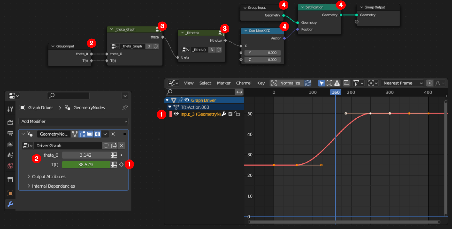
 This picture shows the Geometry Nodes graph coding $f(t)$ as the position of a vertex, and how it is controlled through the Graph Editor.
0. In Object Mode, a mesh made of a single vertex is added, using the Add Mesh Extra Objects Add-ons. Then it is equipped with a GeometryNodes modifier.
1. Keyframes are added to control the $T(t)$ input socket. The shape of the curve $T^n$ as a function of the current frame number $n$ is adjusted in the Graph Editor.
2. $\theta_0$ and $T^n$ are transferred through the Group Input node.
3. $\theta^n$ and $f^n=f(\theta^n)$ are computed using the tool box.
4. The vertex is displaced to the position $(f^n, 0, 0)$. So $f^n$ is exposed outside of Geometry Nodes as the vertex $X$ coordinate.
Driver based on algebra
How to setup as a Driver
How to debug
Resources
Blender file
References

